This is Part 1 of Filtering at scale: how AR’s PostgreSQL design evolved, a series about the table layout, SQL and application code behind audience filtering at Audience Republic.
At Audience Republic, we spent years making audience filtering work against a growing PostgreSQL database. We kept the underlying records separate, but built materialized tables that collected the information needed to search an audience. A lot of the engineering that followed was about the cost of keeping those tables up to date.
Looking back through the server history, the materialization work reaches back to 2017. There are changes to batching, partial updates, locking, indexes and repair paths across the years that followed. It is a much longer story than adding a table to make a query faster.
This first part follows the original filtering approach and introduces the maintenance problems we worked through over time. The next parts will go deeper into how we laid out and indexed the tables, rebuilt selected columns, and made that work hold up under concurrent load, before getting to the newer engine and partitioned tables.
The data model and the question were different shapes
An audience question might combine someone’s profile with their ticket purchases, campaign participation and messaging activity. The records behind those facts have different lifecycles, so keeping them in separate tables makes sense. An order needs to remain an order, with its own status and relationships, regardless of how we want to filter an audience this week.
But the filter has to bring those facts together. Asking for people who attended a particular event and opened a particular message means finding the intersection between different parts of that history.
The materialized tables gave us a representation built for those questions. Instead of reconstructing every relationship for every filter, we could query fields and aggregates that had already been assembled for each fan and promoter.
What that AND/OR toggle asked of the database
The filter builder made this approachable: choose a field, choose a condition, then decide how it combines with the next one. The AND/OR toggle is a small control, but it changes which people belong in the result.
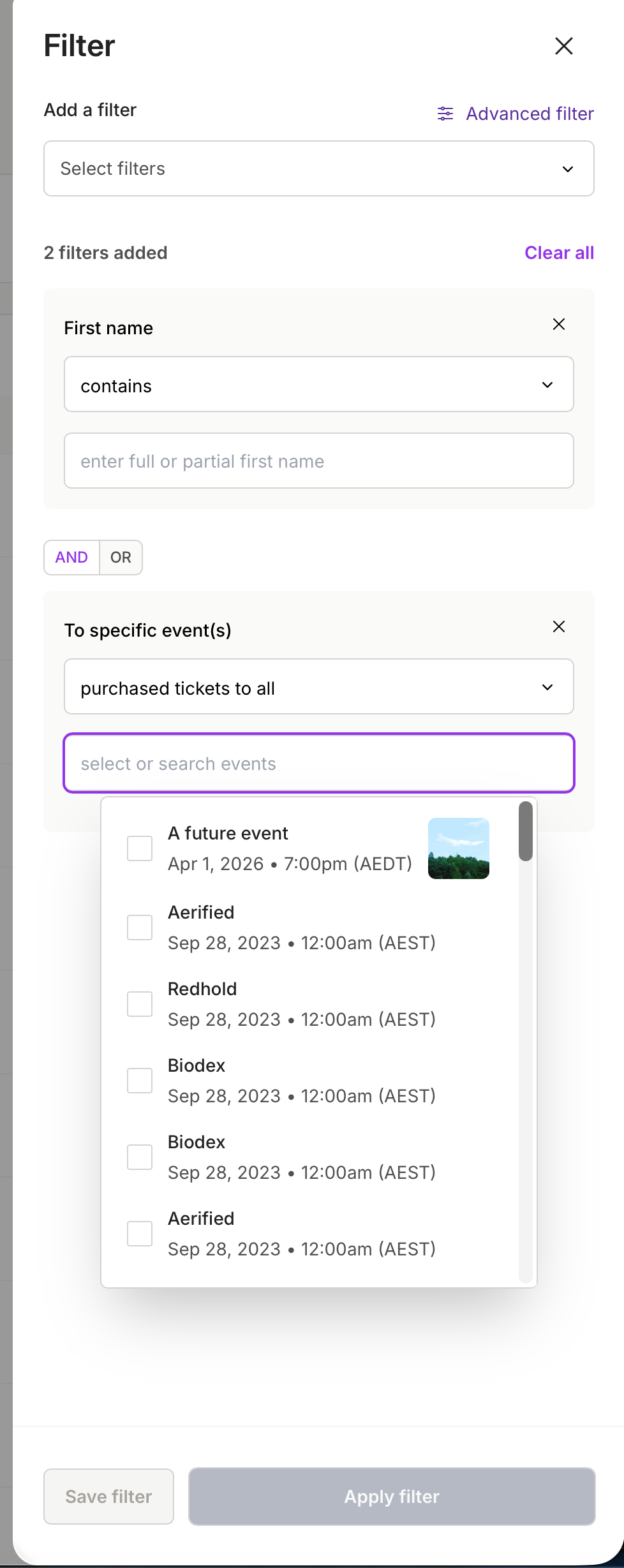
There are two decisions in that screenshot. The AND/OR toggle combines the first-name condition with the event condition. Inside the event condition, “purchased tickets to all” determines whether a fan needs tickets to every selected event, rather than any one of them.
For an illustrative example, suppose we enter “Alex” and select events A and B:
| Choice | Who matches |
|---|---|
| Name contains Alex AND tickets to all selected events | Fans whose name matches and who bought tickets to both A and B. |
| Name contains Alex OR tickets to all selected events | Fans whose name matches, plus anyone who bought tickets to both A and B. |
Changing the outer toggle to OR does not change “all events” into “any event”. Those are separate parts of the expression, and we had to preserve both when generating SQL.
The older implementation carried a list of conditions and a separate list of logic operators. It translated each condition into a SQL predicate, then used an expression parser to assemble the logic and grouping. This is present in the 2021 code, before the newer engine discussed in the follow-up.
For the basic event-membership filter, we had already collected event IDs into the materialized row. The generator selected PostgreSQL’s array containment operator for “all” and its overlap operator for “any”. These simplified predicates show the distinction, using invented event IDs:
-- Bought tickets to both selected events.
mf.events @> ARRAY[101, 202]::bigint[]

-- Bought tickets to at least one selected event.
mf.events && ARRAY[101, 202]::bigint[]
Those are membership tests, not ticket-quantity tests: “all” requires every selected event to be present, but does not exclude fans who also bought tickets to other events. PostgreSQL documents the containment and overlap semantics.
Materialization let us evaluate these combinations against prepared fields instead of rebuilding the underlying purchase relationships for each filter. But it also connected the correctness problem directly to what the user saw: if a purchase changed and we missed the event-array update, a perfectly valid AND/OR expression could still return the wrong audience.
Why we maintained the rows ourselves
We deliberately avoided PostgreSQL’s native materialized-view refresh for this. Refreshing the view meant running its full defining query again, even when the change we needed to reflect affected only a few fields for one fan. CONCURRENTLY allowed reads to continue during that refresh, but it did not let us tell PostgreSQL to recompute just those fields. The PostgreSQL 9.6 documentation describes that full-query refresh behaviour.
Instead, we maintained ordinary tables through SQL functions and application update paths. When we knew which source data had changed, we could focus the work on the affected columns in the materialized row. A change to messaging activity did not inherently require us to rebuild that fan’s unrelated profile or commerce data, let alone refresh the entire audience.
Native view refresh
- Source data changes
- Refresh runs the full query
- Reconcile the view’s result
Application-maintained row
- Source data changes
- Identify affected fan and fields
- Recompute and write those fields
The complication was that we now owned the connection between each source change and the fields it affected. It was possible to save a change correctly in the source tables but miss the corresponding materialization update, leaving the audience filter looking at stale data. That could happen through a missing update path, not just a worker running behind. The narrower updates gave us control over the cost, but made it easier to miss something that a full refresh would have picked up.
Over time, the original materialization approach grew into separate base, messaging, commerce and custom-field tables rather than putting every kind of activity into one increasingly wide row. That gave us somewhere to separate the work, although it only helped when the update paths respected those boundaries too.
Batching helped, but updating less helped as well
The September 2021 benchmark notes have a useful example involving 7,047 fans. They compare individual calls with bulk materialization, including a narrower messaging path for rows that already existed.
| Operation | Individual calls | Bulk |
|---|---|---|
| Full messaging | 52.5 s | 18.7 s |
| Partial messaging updates | 17.9 s | 3.5 s |
| Commerce | 32.2 s | 6.8 s |
Recorded development timings for that workload, not production latency guarantees. Compare results within each row: full and partial messaging perform different work.
That gives us two useful levers. We can process a set of fans together, and we can avoid rebuilding parts of a fan’s materialized data that an event did not affect.
Individual partial updates
Call for fan A → update A
Call for fan B → update B
Call for fan C → update C
Bulk partial update
Call for [A, B, C]
Update the affected set
The later commits are a reminder that getting a better benchmark is not the end of that work. There are fixes for ordering row locks, overlapping updates and falling back to smaller operations when contention became a problem. A batch that runs efficiently by itself still has to coexist with other writers.
In 2023, the history records changes to reduce repeated full-fan materialization around tags and subscriptions. In 2024, another fix removes individual commerce materialization that was happening after a bulk operation had already done the work. These are the kinds of costs that are easy to miss when you only look at the SQL for one call.
The index budget became part of the write budget
Indexes were essential to making the read tables useful. They were also a substantial part of what we had to maintain.
A July 2026 snapshot of the base materialized table recorded about 53 GB of heap data and 273 GB of indexes across 31 indexes. The messaging table had an even larger index footprint in its own July analysis: about 830 GB of indexes against 206 GB of heap data.
| Materialized table | Heap data | Indexes |
|---|---|---|
| Base profile | 53 GB | 273 GB |
| Messaging | 206 GB | 830 GB |
Those are dated snapshots of different tables, not a before-and-after benchmark. They show why it was no longer enough to ask whether another index made a filter faster.
PostgreSQL can avoid creating new index entries for some updates through heap-only tuple updates, usually called HOT updates. That depends on conditions including space on the same heap page and not changing columns referenced by ordinary indexes. An indexed timestamp that changes on every write can therefore be more expensive than it looks. The PostgreSQL HOT documentation explains the conditions.
This is also why changing fewer columns in application code is not a guarantee that we have avoided index maintenance. We need to look at what actually changes, which columns are indexed, and what PostgreSQL reports about the resulting updates.
The index investigations checked both the primary and the read replica. An index with almost no scans on the writer could still be doing useful work on the replica. Constraints and infrequent but important queries also matter, so a low scan count is evidence to investigate, not an instruction to delete.
A sync could do work without changing anything useful
One of the more revealing later findings was that some sync paths recomputed and rewrote materialized rows whether or not their contents had changed.
The July 2026 investigation recorded base-table rewrites at roughly 5.5 times the changes to fan_promoter_account, one of its source tables. That comparison is a warning signal rather than proof that every extra write was unnecessary: the materialized row depends on more than one source. The code inspection was what established the unconditional rewrite path.
The fix added a value-change guard to the bulk base-table upsert. In simplified SQL, the difference looks like this:
-- Before: overwrite the existing value on every conflict.
INSERT INTO read_model AS current (fan_id, country)
VALUES (42, 'AU')
ON CONFLICT (fan_id) DO UPDATE
SET country = EXCLUDED.country;
-- After: leave the row alone if the value is unchanged.
INSERT INTO read_model AS current (fan_id, country)
VALUES (42, 'AU')
ON CONFLICT (fan_id) DO UPDATE
SET country = EXCLUDED.country
WHERE current.country IS DISTINCT FROM EXCLUDED.country;Illustrative SQL against a minimal table, not the full AR schema. The real implementation compares the materialized values across the base row.
IS DISTINCT FROM gives the comparison defined behaviour when either value is null. There was another detail to handle too: sys_mtime is generated afresh, and registration_time has a fallback that can also produce the current time. Including those in the comparison would make unchanged data appear different. The implementation excludes them from the guard.
This does not eliminate the cost of computing the candidate row, and a conflicting upsert can still lock the existing row. It avoids the physical update when the relevant values are equal. That is a narrower claim than “we removed materialization overhead”, but it is a useful boundary to enforce.
What was available when we started
The system’s original design dates to 2016, with the materialization work I found in Git starting in 2017. Keeping a transactional model alongside a different representation for demanding reads was already an established approach. Martin Fowler described separate read and write models in 2011, including the possibility of keeping them in the same database. Our materialized tables fit that family of ideas, although that does not mean the whole application was a CQRS or event-sourced system.
Our choice to maintain selected fields ourselves was deliberate. Native concurrent refresh addressed read availability during a refresh, whereas we needed control over how much data each change caused us to recompute. The cost of that control was maintaining the dependency logic in the application.
Some later tools genuinely were not available at the start. Declarative partitioning arrived in PostgreSQL 10 in 2017, and non-key INCLUDE columns for indexes arrived in PostgreSQL 11 in 2018. Partitioning existed before that through inheritance, but required more machinery. Batching and avoiding duplicate work, on the other hand, were useful then as well. We should not explain every later improvement as something that had to wait for the database to catch up.
What I would build now, and how the newer engine changes these trade-offs, belongs later in the series. Here, the useful starting point is why we chose targeted materialization and what it took to keep it working.
The source of truth still matters
Once you maintain another representation of your data, correctness includes the route between the two. Testing a source update is not enough: we also need to check that it causes every affected materialized field to be updated. Separate workers reaching the same fan introduce another problem, because even correctly identified changes can interfere with one another.
That is why the history contains repair paths and consistency tests alongside performance work. A later bulk-materialization report records zero field mismatches across a 2,500-fan comparison, but it also shows a difficult account improving much less than the others. Equal fan counts do not imply equal amounts of history to aggregate.
I would keep those two questions separate when testing this kind of change: does it produce the same data, and how much work does it do for the accounts that are expensive? An average speedup cannot answer either question on its own.
Keeping the source records normalised gave us a coherent foundation. The materialized tables gave us a way to ask audience questions efficiently. Making that combination work over time meant treating recomputation, freshness, locks and index maintenance as part of the design, rather than overhead we would deal with later.
Filtering at scale: how AR’s PostgreSQL design evolved
There is enough history here for several articles. This is the outline I’m working through; the remaining parts are planned, and I’ll add links as they’re published.
- The original read model — this article. Why we kept the source data normalised and assembled a different representation for filtering.
- How we laid out the tables, and what the indexes cost — planned. Separating profile, messaging, commerce and custom-field data, then balancing faster filters against the work each write creates.
- Rebuilding the columns that actually changed — planned. A SQL and application-code deep dive into source-to-column dependencies, partial updates, bulk operations and avoiding writes when the values haven’t changed.
- Keeping rebuilds correct when the system is busy — planned. Overlapping updates, lock ordering, batch sizes and repair paths, with the measurements and consistency checks needed to judge whether an optimisation holds up under load.
- How the filtering engine evolved — planned. The newer engine and partitioned tables, what changed as the workload grew, and which choices I would revisit if we were starting today.
The deeper dives will follow the code changes and recorded database measurements over time, with before-and-after SQL and diagrams to show how a source change reaches the materialized columns.